Demystifying Gradient Descent for Simple Linear Regression in Python

1. Introduction

In this blog post, we will walk you through the process of implementing gradient descent for a simple linear regression problem using Python. Simple linear regression is a fundamental machine learning technique that aims to model the relationship between two continuous variables. Gradient descent is an optimization algorithm that helps find the optimal values for the model parameters by minimizing the cost function.

2. Prerequisites

To follow along with this tutorial, you should have:

• Basic understanding of Python programming
• Familiarity with NumPy and Matplotlib libraries

3. Dataset

We will use a small synthetic dataset (x = [1, 2, 3, 4, 5], y = [3, 4, 5, 6, 7])

to demonstrate the implementation of gradient descent for simple linear regression. Feel free to replace it with your dataset.

4. Implementing Gradient Descent

4.1. Define the cost function

We start by defining the cost function (Mean Squared Error), which measures how well our line fits the data. Our goal is to minimize this value.

def cost_function(m, b, x, y):
    n = len(x)
    total_error = np.sum((y - (m * x + b))**2)
    return total_error / n

4.2. Compute the gradients

We calculate the partial derivatives of the cost function with respect to m and b, which indicate how much the error will change as we update m and b.

def gradients(m, b, x, y):
    n = len(x)
    dm = -(2/n) * np.sum(x * (y - (m * x + b)))
    db = -(2/n) * np.sum(y - (m * x + b))
    return dm, db

4.3. Update the parameters

We iteratively update m and b by moving in the opposite direction of the gradients, which leads to the minimum of the cost function.

def gradient_descent(m, b, x, y, learning_rate, iterations):
    for _ in range(iterations):
        dm, db = gradients(m, b, x, y)
        m -= learning_rate * dm
        b -= learning_rate * db
    return m, b

4.4. Test the algorithm

Apply the gradient descent algorithm to the dataset and print the optimal values of m and b.

m_init, b_init = 0, 0
learning_rate = 0.01
iterations = 1000

m_optimal, b_optimal = gradient_descent(m_init, b_init, x, y, learning_rate, iterations)
print(f"Optimal m: {m_optimal}, Optimal b: {b_optimal}")

5. Visualizing the Results

We can visualize the results using the matplotlib library in Python. Create a scatter plot of the data points, and then plot the best-fit line obtained from the gradient descent algorithm.

def plot_regression_line(x, y, m, b):
    plt.scatter(x, y, color='blue', label='Data points')
    
    # Calculate the predicted values using the optimal m and b
    y_pred = m * x + b
    
    # Plot the best-fit line
    plt.plot(x, y_pred, color='red', label='Best-fit line')
    
    # Add labels and legend
    plt.xlabel('x')
    plt.ylabel('y')
    plt.legend()
    
    # Show the plot
    plt.show()

# Call the function to plot the regression line
plot_regression_line(x, y, m_optimal, b_optimal)

6. Cost Function Visualization

To visualize the cost function landscape and the optimization process of gradient descent, we can create a 3D plot with the cost function values for different combinations of m and b.

def plot_cost_function(x, y, m_optimal, b_optimal):
    m_values = np.linspace(m_optimal - 2, m_optimal + 2, 100)
    b_values = np.linspace(b_optimal - 2, b_optimal + 2, 100)
    
    M, B = np.meshgrid(m_values, b_values)
    cost = np.array([cost_function(m, b, x, y) for m, b in zip(np.ravel(M), np.ravel(B))]) Cost = cost.reshape(M.shape)

fig = plt.figure()
ax = fig.add_subplot(111, projection='3d')

ax.plot_surface(M, B, Cost, cmap='viridis', alpha=0.8)
ax.scatter(m_optimal, b_optimal, cost_function(m_optimal, b_optimal, x, y), c='red', marker='o', s=100)

ax.set_xlabel('m')
ax.set_ylabel('b')
ax.set_zlabel('Cost')

plt.show()

Call the function to plot the cost function

plot_cost_function(x, y, m_optimal, b_optimal)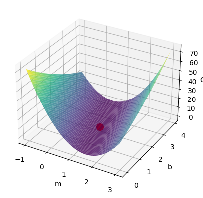

Conclusion

In this tutorial, we demonstrated how to implement a simple linear regression model using gradient descent in Python. By understanding the underlying concepts and visualizing the results, we can better grasp the optimization process and the relationship between the model parameters and the cost function. I hope this step-by-step guide has provided you with a solid foundation for implementing gradient descent for simple linear regression problems. If you want to build your own model, fork the repo here on GitHub.